


[ad_1]
In the previous post, we gave an overview of Cinnamon and its different components. In this second part we’ll dive into the rejector and specifically how we use PID controllers to make a mean and lean rejector.
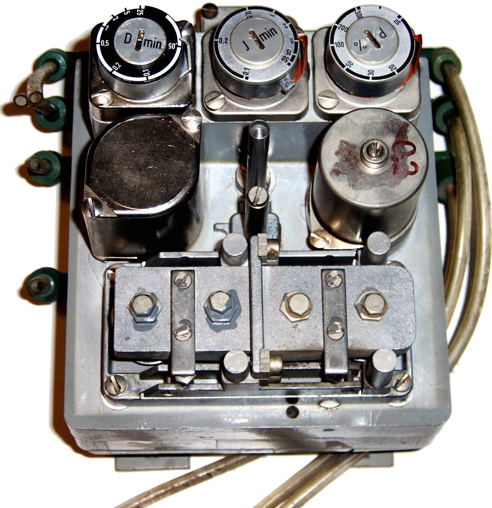
A PID controller is a control-loop mechanism that, given some feedback, continuously tries to make a calculated error value, called the target function, go to zero. Its basis has been known for over 300 years, and the mathematical formulation was given in 1922. It is widely used in the industry, where it controls anything from the temperature in an oven to steering a ship. And it turns out that they excel in quickly calculating a stable rejection ratio for load shedders (something we have not achieved with alternatives such as AIMD and CoDel).
The challenge for Cinnamon has been to find a good target function for the PID controller that is portable between services without config changes. As examples, we have some services at Uber where a single instance is processing thousands of requests per second (RPS) and we have some that process 10 RPS per instance. Given the sheer number of microservices, we really want something that does not require configuration. This blog post will describe this target function, how we arrived at it and how it performs in practice.
Introduction
To recap, the diagram below shows the Cinnamon architecture, and this post will dive into the area marked by the red box:
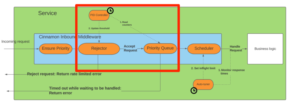
The main goal of the rejector is to determine how many requests to reject when the endpoint is overloaded. We want the ratio to be fairly stable, as we otherwise easily get oscillating latencies. Thus it needs to adapt to the patterns of the service to set threshold. Lastly, because Cinnamon logic is involved by all requests, the overhead has to be minimal (both in terms of latency added and resources consumed).
In the following we describe how all three goals are achieved by leveraging PID controllers.
Architecture
The rejector uses two parts: a) the online part that simply rejects or accepts each request based on their priority, and b) an offline part that runs every so often (typically every 500 ms) and recalibrates the threshold.
The online part is very efficient as it only needs to read the priority of the request and compare it with an atomic integer containing the threshold. If the priority is higher than the threshold, we accept the request, otherwise we reject it.
The offline part does the heavy lifting of figuring out if an endpoint is overloaded and if so, calculating what percentage of requests should be load shedded. The calculated percentage is afterwards converted to a priority threshold by inspecting the last 1,000 requests the endpoint has seen. By dynamically recording the priorities of the requests seen, Cinnamon automatically adjusts the threshold to changing traffic patterns (even if the percentage is the same).
To find the percentage over requests to load shed, Cinnamon uses a PID controller over the following two values (and we’ll describe it next):
- The incoming requests to the priority queue
- The outgoing requests from the queue and into the service to be handled
Context: PID Controller
Before diving into how Cinnamon uses the PID controller, we want to briefly describe how they work in general (feel free to skip ahead if you are already familiar).
Imagine the cruise control in a car, where its job is to figure out how much power the engine needs to go from your current speed to a target speed (e.g., 20 to 80 km/h). The power to apply very much depends on how fast you’re going right now (e.g., at 20km/h it should accelerate more than when you’re driving 70 km/h). Once your car hits 80km/h, it should ideally stay around the power it is applying to the engine currently. A PID controller is ideal in this case, as it dynamically adjusts the power to apply, even when the road conditions change (e.g., going uphill/downhill).
A PID controller consists of three parts/terms (a proportional, integral and derivative), where:
- Proportional is the difference between the target value and the current value. Thus the further away the current value is from the target value, the larger the P term will be.
- Integral is the sum of the historic P values. In the example above, when the cruise control hits the 80km/h, the P value will be zero, but the I part will be non-zero and thus ensure that the car still applies power to the engine to keep the car at 80km/h.
- Derivative is the rate of change of P. Thus if P changes a lot, D helps to dampen the effect a bit. (We won’t spend time on D here, as we did not find it useful for Cinnamon).
The PID value at a given time is then a weighted sum of the three terms above, where the weight of each term is typically called Kp, Ki, and Kd. This feedback loop is shown in the block diagram below, and how we use it in Cinnamon (in high-level terms):
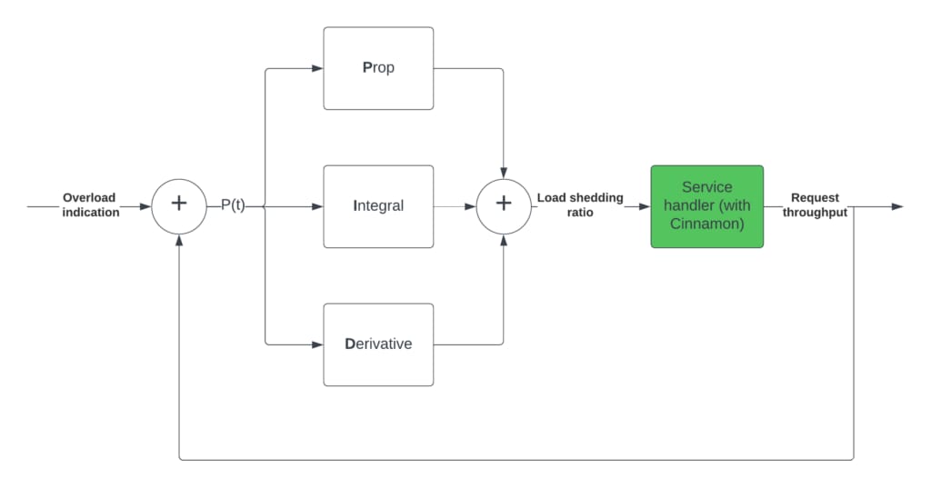
The idea is that when a service is overloaded, we use the request throughput to calculate the P(t), that is then used to calculate the P, I and D terms. The result of that value is feed into Cinnamon (inside the service), which affects the request throughput (and is thus feed back into the PID).
If you are interested in the mathematical description of the above, we highly recommend the Wikipedia article on PID controllers. Note that in the mathematical formulation of PID controllers, the integral is the sum of the full history, whereas with Cinnamon, we bound it to the last 30 seconds, to limit the overlap of different query patterns, but otherwise Cinnamon follows the above.
Figuring Out The Percentage
Returning back to Cinnamon, the goal of its PID controller is to control the rejection percentage such that:
- It keeps the outstanding queue at a minimum, thus minimizing queue time
- It keeps the number of concurrently executing requests at the limit, thus fully utilizing the service
If we only had 1 as a goal, then you could easily come up with a rejector that would reject all requests but one. That way there is no queueing time, but you severely limit the throughput of the service. Including 2 into the PID controller means it has some backpressure if the PID overshoots and rejects too much. Compared with a cruise control, if its PID controller overshoots and applies too much power to the engine, the excess speed will also put backpressure into the PID controller.
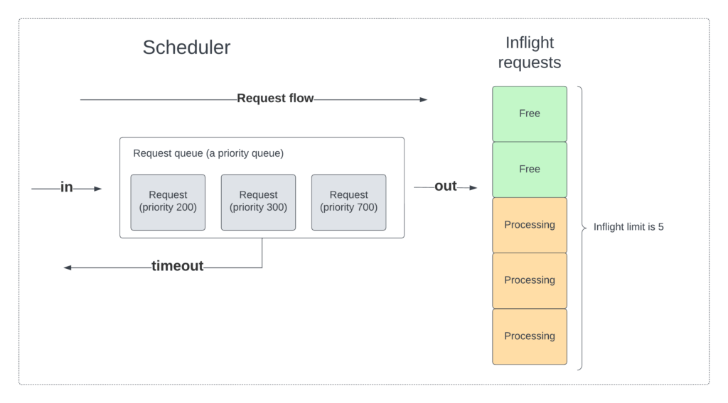
The picture below shows the relationship between the request queue and the inflight requests. In this case the inflight limit is five (thus, five requests can be handled concurrently), where only three are being processed. Further we have three outstanding requests. Thus this case violates both above, namely that we don’t fully utilize the inflight limit and we have outstanding requests. Note that the PID controller has nothing to do with estimating the inflight limit, that is the job of the auto-tuner, which will be described in the next blog post.
With the above in mind, we use the following to calculate the P value for Cinnamon:
- t denotes a time period (e.g., 500ms)
- in(t) is the total number of requests going into the request queue in the calibration period (note this number only includes accepted requests and not the ones that were rejected by the rejector, displayed by in in the diagram above)
- out(t) is the number of requests exiting the queue in the calibration period (thus are to be handled by the service, displayed by out in the diagram above)
- freeInflight(t) is the difference between the current number of inflight requests and the inflight limit (displayed by the green boxes in the above diagram)
- out'(t) is identical out(t), except if out(t) is zero, then out'(t) is equal to inflightLimit
If we break it down, the intuition is fairly straightforward. Ideally, in a given time period we want the number of requests going into the queue to be the same as the number of requests being pulled out of the queue and forwarded to the service (in other words, going inflight). Thus, we arrive at the following initial equation:
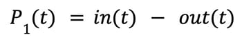
This first version says that if P1(t) is positive (i.e., in > out) we need to load shed more, as the queue is growing. On the other hand, if P1(t) is negative (i.e., in < out), then the service is emptying the queue (which is good), but it indicates that we might be load shedding too much. The above version does not, however, take the utilization of the service into account. For example, if in and out is 5, then P1(t) is zero, and according to the equation we load shed as we should. But, if only 1 request goes inflight at any time and the limit is 5, we have unused capacity. Thus in the next iteration, we extend the above to take into account the number of unused inflight spots, also called freeInflight:
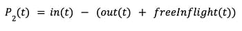
In this case, if in(t) and out(t) is the same value and freeInflight(t) is zero, we have the ideal case, where the service is fully saturated and we have the same number of requests entering the queue as is exiting it. On the other hand, if freeInflight(t) is non-zero and in(t) and out(t) are the same, the P value would be negative and reduce load shedding, as it should (we’re essentially rejecting too much).
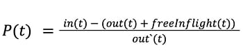
The last step in the above is to take into account that different services are handling a wide spectrum of RPS. If say in(t) – out(t)=1 for a service instance handling, for instance 1,000 RPS, you should not load shed as much (if any) compared if the service instance is doing 1 RPS. Thus, we normalize the P value with the number of requests in the period, which equals out(t). There is one caveat – namely that there might be periods where no requests have been processed, and then we use inflightLimit as an estimate of the normalizer. Therefore, you arrive at the following equation:
One thing to note is that the equation does not explicitly mention the number of timeouts happening in the queue, as it is implicitly handled in the difference between in(t) and out(t). Another thing you might wonder is what if in is higher than out and freeInflight is non-zero, then the P value can be zero (and thus seen as adequate). This is not a problem, because when in is larger than out and there are free inflight spots, the surplus of incoming requests should be quickly assigned an inflight spot, which means in the next recalibration period, the freeInflight will be zero.
From an implementation perspective, the above can be done very efficiently. You just need two atomic counters in the hot path that are incremented when a request enters the queue and it exits and is forwarded to the service code itself. That way the background recalibration should store the last seen values of these two counters and can calculate the number since the last recalibration period.
The P value function defined is calculated whenever the recalibration is run and we plug it into the PID controller, including adding it to the history. In comparison with a standard PID controller, we’ve modified the integral over the history a bit to make it a bounded history. Normally, the integral part of a PID controller should be for the full interval (e.g., for a cruise control, it is calculated from when you start the cruise control), but for load shedding we’ve noted that each load shedding case can be different and thus using a bounded history reduces overlap between consecutive overloads and better adapts to changing request patterns. Typically we bound it to 30 seconds.
In order to find the Kp and Ki constants for the PID equation, we ran a days-long test, where we incrementally changed both and ran a load test and then inspected the results. From that we found that Kp = 0.1 and Ki = 1.4 worked the best. There are many more methods we could have used, but so far the above has worked well.
Ratio To Threshold
From the PID controller’s ratio, the rejector must calculate the priority threshold that needs to be shedded (remember that a request has a priority, which we have to compare against). And in order to do that, we keep track of the last, say, 1,000 requests and their priority (with 1,000 we get a good sample of traffic, even if it is a high RPS endpoint). Say the PID regulator sets the threshold to 10%, we can use the cumulative priority of the last 1,000 requests to deduce the threshold, as shown in the (example) diagram below:
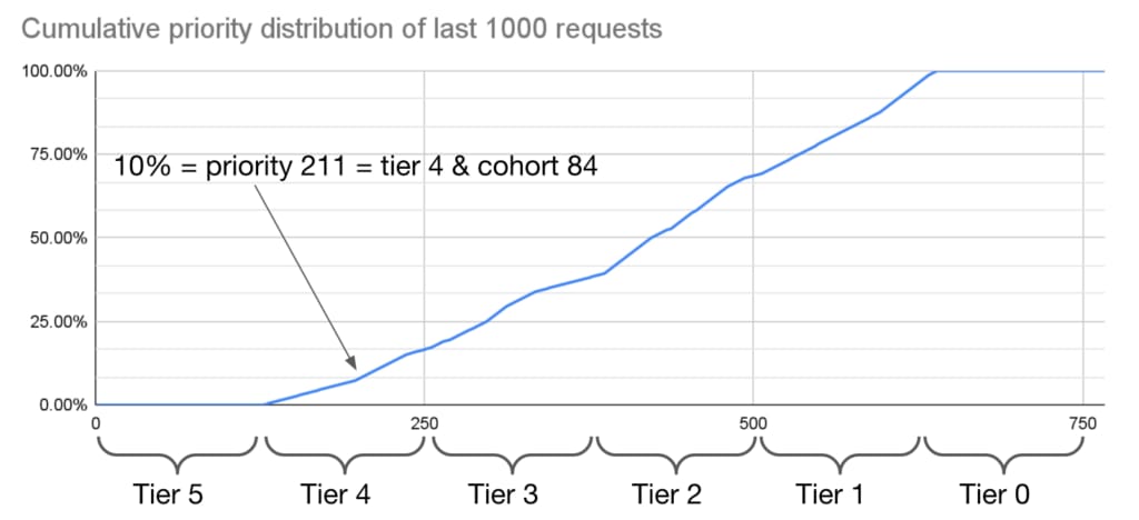
For this service, which has seen an equal amount of tier 1 to tier 4 requests, the 10% threshold equals tier 4 and cohort 84.
Experiment
In the first blog post, we have already shown that Cinnamon is able to sustain a stable rejection rate, even as the auto-tuner changes the inflight limit. Thus, here we want to focus on the PID controller and see how fast it can change the rejection rate (both up and down) as load changes.
More specifically, we want to test the PID controller by sending various amounts of traffic to the service and then monitor how fast the PID reacts and how fast it achieves a stable rejection limit. To do so, we reuse the same test setup as in blog post 1, where the test service is distributed over two backend nodes and is able to handle ~1,300 RPS in total. In order to just describe the effect of the PID controller, we have disabled the auto-tuner and manually set the inflight limit. We send a base load of 1,000 RPS, and then at various times send more RPS to go above the limit.
The result of this experiment is shown in the graphs below (carried out over ~25 mins). The top graph shows the total inbound RPS (yellow line) and the goodput/accepted RPS (green line). The bottom one shows a histogram of the rejection rate, where each instance emit a data point every 500 milliseconds. One important aspect of these graphs is that the underlying time series database (M3) has a minimum resolution of 10 seconds, which means that for the rejection rate graph, all data points are grouped in 10 seconds intervals, which you can see as point “towers.”
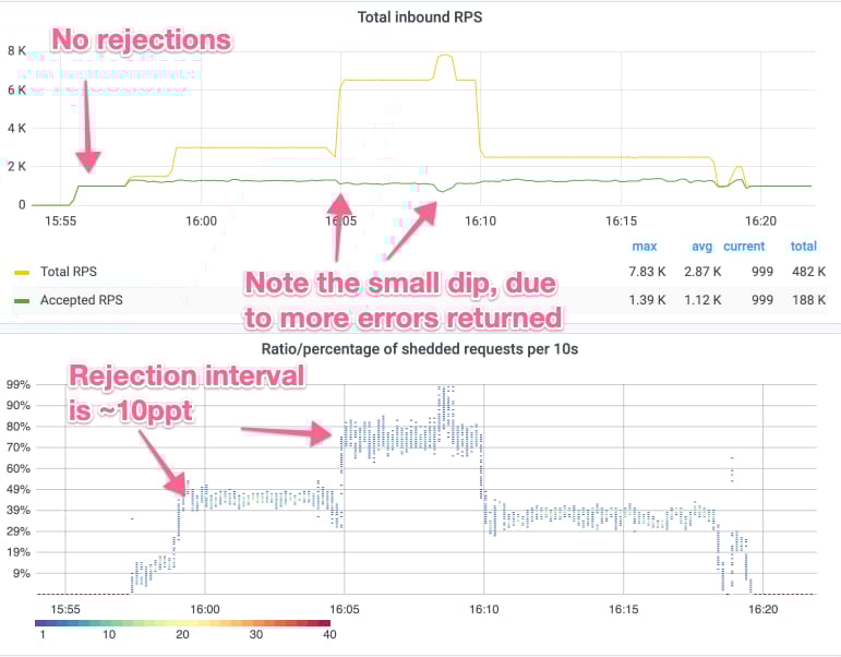
As an example, at 16:05 in the diagram above, we increase the load from ~3,000 RPS to ~6,500 RPS (yellow-line), of which ~1,300 RPS are accepted (green line), and the rest rejected. With the increased load the rejection rate quickly goes from ~30% to ~75%, and it only takes 10 seconds (and likely less, but we can’t see that because of the time resolution). Lastly, after the load increases, the rejection rate quickly stabilizes between 70% and 80%. We call this 10 percentage points (a.k.a., ppt) interval for the rejection span and as can be noted, the rejection span is ~10ppt for all the steady states of incoming RPS.
The interesting aspect of this is, that even though the rejection span for a given RPS is around 10 percentage points, the span does not increase when Cinnamon has to reject a lot of the traffic. When we experimented with other mechanisms (e.g., AIMD or CoDel), we would typically get a narrow rejection span, when the rejection ratio was small, but then a huge rejection span (e.g., 30ppt) at large rejection ratios (e.g., >50%). We believe that the history component of PIDs is crucial for these stable rejection intervals, as it remembers what we have done so far, and thus avoids oscillating between rejecting everything and rejecting nothing (which CoDel is prone to).
Summary
By using a PID controller, Cinnamon is able to quickly react to load changes during overload and more importantly, is able to find a stable ratio to load shed, that ensures the request queue is kept short, while best utilizing the resources of the service. Furthermore, we have seen that the PID controller works well for both low-traffic and high-traffic services, where we normally see a rejection span around ~10ppt (this was not the case with earlier iterations of the PID controller).
Figure 1 Image Attribution: CC BY-SA 3.0 and is credited to Snip3r (via Wikipedia)
[ad_2]
Source link

